This project seeks to analyze the sentiment of 8-Ks for each year-quarter from the SEC webite from 1995-2018. The goal is to see if any correlation exists between the sentiment, or tone, of the 8-K and the subsequent abnormal trading volume or abnormal returns around the actual event date. This task is divided into three parts: 1. Downloading the Data, 2. Event Studies, 3. Rudimentary Sentiment Analysis, and 4. Advanced Sentiment Analysis.

1. Downloading the Data

There were a few main sources of data used for this project:

a. 8-K Texts : This was downloaded from the SEC webside, and all 8-Ks starting from 1995 Q1 to 2018 Q4 was obtained, and each company was labeled by their unique CIK number. For each quarter, 100 random 8-K’s were selected to analyze. This results in over 9500+ documents to analyze.

b. DSF : The daily stock returns and volume, along with shares outstanding, were obtained by analyzing the DSF SAS file which was obtained through the QCF server. This data file had company information in the form of the CUSIP number.

c. FUNDA : This company-specific data information file contained the link between CUSIP and the CIK number, which was used to relate the 8-K texts to the DSF data file. This document was found as well through the QCF server.

d. Bill McDonald’s Word List : This data file assigned a positive and negative value to each word, and it was used to determine the overall tone in the rudimentary sentiment analysis.

In actually downloading the data, Python was used for the data extraction to grab the information from each URL, specifically using the ‘requests’ module. Since each of the 8-K’s was in the form of an html script, the module ‘Beautiful Soup’ was used in order to parse through the html and only grab the body of the document.

The Python script can be seen in the GitHub pages as ‘sentimentAnalysis.py’. It was put here because the code runs more smoothly to go ahead an perform the Sentiment Analysis in the next sections while downloading the data.

Event Studies

This task sought to look at the CIK and filing date pair from the previous section to determine the cumulative abnormal return (CAR) and cumulative abnormal volume (CAV) for each CIK/filing date pair. The abnormal return (AR) is defined as the return in excess of the CAPM market return, regressed from -315 to -91 days from the event or filing date. The ‘cumulative’ part of the definition arises from summing the rolling window of abnormal returns around the event date. For instance, the three-day window consists of the day prior to the event date, the event date, and the day after the event date. The one-day, three-day, and five-day rolling window was calculated for both CAR and CAV.

We can define the CAV as the normalized trading volume, calibrated to -71 to -11 days before the event date and taken on a log scale. For clarification, suppose the range of -71 to -11 days was not quite a volatile range of trading, while the cumulative three-day rolling window around the event date was very volatile, then the CAV would be a large number, scaled by a standard deviation or more from the mean of the past -71 to -11 day rolling window.

The table below shows the descriptive statistics for the CAR and CAV rolling windows over the sample period 1995:2018.

—	CAR(1)	CAR(3)	CAR(5)	CAV(1)	CAV(3)	CAV (5)
Mean	-0.001508	-0.002782	-0.003579	0.526526	1.206844	1.863234
Standard Deviation	0.061269	0.096360	0.124626	1.513595	3.473083	6.329492
Minimum	-0.732448	-0.807893	-0.934338	-8.344340	-19.990874	-27.465825
25%	-0.018018	-0.029812	-0.043501	-0.423825	-1.007499	-2.104361
50%	-0.000766	-0.001695	-0.002122	0.387644	0.844627	1.365758
75%	0.014817	0.024814	0.035890	1.236411	2.974241	5.078070
Maximum	1.105913	1.936429	1.787982	12.774111	23.541118	42.558456

Additionally we can plot the distribution of both measures, given first by the cumulative abnormal return (CAR):

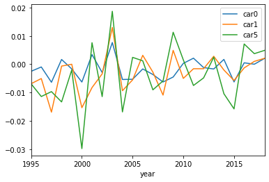
Notice what this might be saying: from 1995-2018, the CAR trends slightly upward and is definitely non-zero, meaning the returns experienced over the event date are slightly different than what the CAPM model would suggest. However, considering the mean is roughly zero, this indicates the CAPM does a fairly good job at predicting returns.

For the cumulative abnormal volume, the distribution is given by:

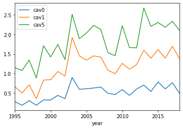
Notice here one interesting tidbit, is the CAV has a slight trend upwards, possibly indicating the volatility in the future is greater than the past would predict.

This Python script can be seen in the GitHub pages as ‘eventStudies.py’. Be cautioned though, this code takes around ~1hr to run, because of the intensive process in calculating the CAV and CAR for each event study.

This code produces the final ‘sentimentAnalysisAndEventStudies.csv’ data file to obtain all information for each event study.

Rudimentary Sentiment Analysis

The main task for this section was to compute the abnormal stock returns and abnormal trading volume around 8-K filings, and study how these measure vary depending on the number of positive and negative words included in the filing.

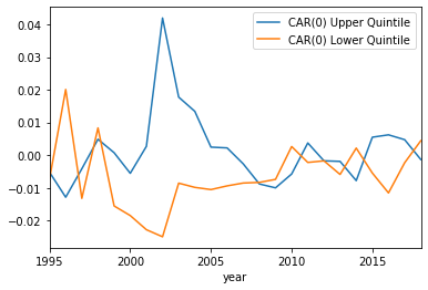
In obtaining the positivity and negativity of the document, these results can be sorted into quintiles. If we calculate the descriptive statistics for the CAR and CAV in the highest vs. lowest percentile, we obtain the following charts:

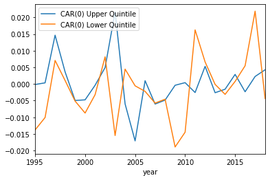
CAR(0) plotted with the upper and lower quintiles:

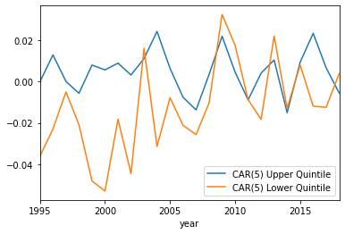
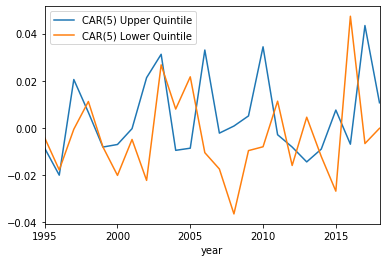
CAR(5) plotted with the upper and lower quintiles:

CAV(0) plotted with the upper and lower qunitiles:

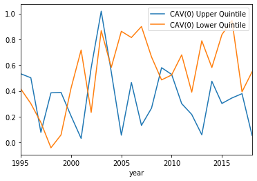
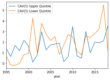
CAV(5) plotted with the upper and lower quintiles:

These results are very interesting! It seems the sentiment of the 8-K from this rudimentary analysis doesn’t capture the overall effect of CAR and CAV, because it is hard to see any trend. The upper and lower quintiles seems to follow the same general pattern, except for a few exceptions or so. The one noticeable difference is in the CAR(0) upper quintile around 2001. This may simply be due to some noise, but it is remarkably higher in this time period. Could this be some effect due to the ‘dot com’ bubble burst of 2000? It is not clear, as an analysis of the more robust sentiment analysis could give more insight.

This Python script can be seen in the GitHub pages as ‘sentimentAnalysis.py’, and is combined with the section below.

Advanced Sentiment Analysis

In this section, a more thorough analysis of the ‘tone’ of the 8-K is performed by looking at the tonality of each sentence in the document, rather than merely counting positive and negative words. The natural language toolkit provided by the ‘NLTK’ module in Python was an excellent resource to complete this task.

The first thing to notice in this section is difficult in cleaning up an html file. Even with the best tools, it can sill be an imprecise tool. However, how I went about this task was to clean the html string in a series of steps:

1. Use the ‘BeautifulSoup’ module to remove all white spaces in the document and only extract the body of the html file.
2. Use the ‘RegexpTokenAnalyzer’ function in the NLTK toolkit to grab only words and words which ended with a standard sentence ending (.!?).
3. Use the ‘sent_tokenize’ function in the NLTK toolkit to split the string into sentences.
4. Assign a tonality to each sentence by the ‘ ‘ function in the NLTK toolkit to analyze the tonality of each sentence.
5. Sum up the overall tonality and divide by the total number of sentences to grab the offical ‘tone’ of the 8-K.

After this, it was relatively easy to sort the 8-K documents into quintiles and generate the descriptive statistics for the upper and lower quintile. Specifically, when calculating the mean, the result is:

CAR(0) plotted with the upper and lower quintiles:

CAR(5) plotted with the upper and lower quintiles:

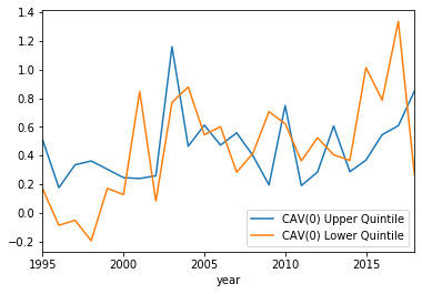
CAV(0) plotted with the upper and lower qunitiles:

CAV(5) plotted with the upper and lower quintiles:

The results seem a little underwhelming. By and large it seems the sentiment of the 8-K plays little role in actually generating abnormal returns, except for a few years. However, it is hard to tell which years these will be, as some years the lower quintile has a larger abnormal return, and some years the upper quintile has the larger abnormal return.

Some descriptive statistics are given in the following table for the five-day rolling window:

—	CAR(5) Upper	CAR(5) Lower	CAV(5) Upper	CAV(5) Lower
Mean	0.00460	-0.00407	1.6278	1.9775
Standard Deviation	0.10961	0.12776	5.90024	6.9308

This chart highlights what was seen in the plots above. There is a slight advantage to a more positive tone to the 8-K, by almost 1%. However, by looking at the time series data, it is hard to discern when this will happen. All which can be said is, on average, there is a slight advantage to a more positive tone in the 8-K. So talk positive!

This Python script can be seen in the GitHub pages as ‘sentimentAnalysis.py’. Be cautioned though, this code takes around ~1hr to run, due to the time-intensive process of analyzing each 8-K.

This code produces the ‘sentimentAnalysis.csv’ data file, which is used by the ‘eventStudies.py’ script in order to obtain the final output.